Karenina¶

Simulation and modeling tools for studying Anna Karenina effects in animal microbiomes This package aims to develop tools for modeling microbiome variability in disease. Initial versions focus on simulating microbiome change over time using simple Ornstein-Uhlenbeck (OU) models.

Happy families are all alike; every unhappy family is unhappy in its own way.: Leo Tolstoy

Links¶

Installation¶

Karenina is in active development and is available as a direct command-line program (karenina), or as a Qiime2 plugin (q2-karenina). Karenina is a python3.5+ program and requires scipy, pandas, matplotlib, and seaborn.

Install ffmpeg (visualization dependency)

sudo apt-get install ffmpeg -y

Install karenina

pip install git+https://github.com/zaneveld/karenina.git

Qiime2 Users¶

Qiime2 users will have the ability to use their Q2 Artifacts and receive output compatible with other Q2 plugins. q2-karenina requires both ffmpeg and karenina.

Install q2-karenina

pip install git+https://github.com/zaneveld/q2-karenina.git

Update Qiime2 cache to enable newly installed plugin.

qiime dev refresh-cache

Usage¶

Script	Description
spatial_ornstein_uhlenbeck	OU Simulation Modeling
fit_timeseries	Fit PCoA Data to OU Models
karenina_visualization	Visualize PCoA Timeseries
qiime karenina spatial-ornstein-uhlenbeck	Q2 application of OU Modeling
qiime karenina fit-timeseries	Q2 application of PCoA fitting
qiime karenina visualization	Q2 application of 3D Visualization

karenina¶

spatial_ornstein_uhlenbeck¶

>spatial_ornstein_uhlenbeck -h

Usage: spatial_ornstein_uhlenbeck -o ./simulation_results

This script simulates microbiome change over time using Ornstein-Uhlenbeck
(OU) models.  These are similar to Brownian motion models, with the exception
that they include reversion to a mean. Output is a tab-delimited data table
and figures.

Options:
  --version             show program's version number and exit
  -h, --help            show this help message and exit

  Required options:
        -o OUTPUT, --output=OUTPUT
                                                the output folder for the simulation results

  Optional options:
        --pert_file_path=PERT_FILE_PATH
                                                file path to a perturbation file specifying parameters
                                                for the simulation results
        --treatment_names=TREATMENT_NAMES
                                                Comma seperated list of treatment named
                                                [default:control,destabilizing_treatment]
        -n N_INDIVIDUALS, --n_individuals=N_INDIVIDUALS
                                                Comma-separated number of individuals to simulate per
                                                treatment.Note: This value must be enclosed in quotes.
                                                Example: "35,35". [default: 35,35]
        -t N_TIMEPOINTS, --n_timepoints=N_TIMEPOINTS
                                                Number of timepoints to simulate. (One number, which
                                                is the same for all treatments) [default: 10]
        -p PERTURBATION_TIMEPOINT, --perturbation_timepoint=PERTURBATION_TIMEPOINT
                                                Timepoint at which to apply a perturbation. Must be
                                                less than --n_timepoints [default: 5]
        -d PERTURBATION_DURATION, --perturbation_duration=PERTURBATION_DURATION
                                                Duration that the perturbation lasts. [default: 100]
        --interindividual_variation=INTERINDIVIDUAL_VARIATION
                                                Starting variability between individuals. [default:
                                                0.01]
        --delta=DELTA       Starting delta parameter for Brownian motion and
                                                Ornstein-Uhlenbeck processes. A higher number
                                                indicates more variability over time. [default: 0.25]
        -l L, --L=L         Starting lambda parameter for Ornstein-Uhlenbeck
                                                processes. A higher number indicates a greater
                                                tendancy to revert to the mean value. [default: 0.2]
        --fixed_start_pos=FIXED_START_POS
                                                Starting x,y,z position for all points, as comma
                                                separated floating point values, e.g. 0.0,0.1,0.2. If
                                                not supplied, starting positions will be randomized
                                                based on the interindividual_variation parameter
                                                [default: none]
        -v, --verbose
                                                allows for verbose output [default: False]

The spatial_ornstein_uhlenbeck function takes in simulation parameters and develops a distance matrix, PCoA ordination, and metadata file for use in other processes. This tutorial will explore the functionality of the script, and provide sample input data for fit_timeseries and karenina_visualization.

The following parameters are used to generate a simulation using Ornstein Uhlenbeck and Brownian motion models:

-o [Direct/filepath/to/output/dir/]
--n_timepoints 50
--perturbation_timepoint 15
--n_individuals 3,3

The following parameters were used as their default input:

--treatment_names control,destabilizing_treatment
--pert_file_path os.path.abspath(resource_filename('karenina.data','set_xyz_lambda_zero.tsv'))
--perturbation_duration 100
--interindividual_variation 0.01
--delta 0.25
--L 0.20

After installing karenina, the following command is used to execute the simulation from within the output directory.

spatial_ornstein_uhlenbeck -o ./ --n_timepoints 50 --perturbation_timepoint 15 --n_individuals 3,3

This generates the following files:

ordination.txt : Simulation PCoA data
metadata.tsv : Simulation metadata file
log.txt : Simulation parameters
euclidean.txt : Euclidean distance-matrix of Simulation data
simulation_video.mp4 : Visualization of simulated data

These files can be viewed here:

https://github.com/zaneveld/karenina/tree/master/data/outputs/OU_simulation_50.3.3

fit_timeseries¶

>fit_timeseries -h

Usage: fit_timeseries -o ./simulation_results

This script fits microbiome change over time to Ornstein-Uhlenbeck (OU)
models.Demo fitting an OU model using default parameters.

Options:
  --version             show program's version number and exit
  -h, --help            show this help message and exit

  Required options:
        -o OUTPUT, --output=OUTPUT
                                                the output folder for the simulation results

  Optional options:
        --fit_method=FIT_METHOD
                                                Global optimization_method to use
                                                [default:basinhopping]
        --pcoa_qza=PCOA_QZA
                                                The input PCoA qza file
        --metadata=METADATA
                                                The input metadata tsv file, if not defined, metadata
                                                will be extracted from PCoA qza
        --individual=INDIVIDUAL
                                                The host subject ID column identifier, separate by
                                                comma to combine TWO columns
        --timepoint=TIMEPOINT
                                                The timepoint column identifier
        --treatment=TREATMENT
                                                The treatment column identifier
        -v, --verbose
                                                allows for verbose output [default: False]

The fit_timeseries process allows users to fit PCoA and Metadata information to Ornstein Uhlenbeck models.

Warning

This script does not allow for optimization of single-point observations, where individuals are only measured or treated at one specific timepoint. If subjects are applied treatments at a single timepoint, it may be necessary to manually modify the metadata file to apply a boolean label to “treatment x applied” or not.

Note

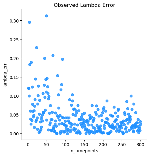
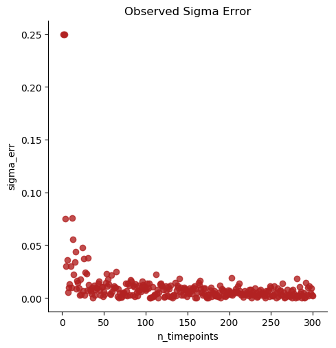
The optimal number of measured timepoints is roughly 50 per subject, based on benchmarking.

Using the data from the previously ran simulation (see spatial_ornstein_uhlenbeck), the fit_timeseries process will attempt to fit Ornstein Uhlenbeck models to the individuals and treatment cohorts of the input data.

The data being used for this tutorial can be found here:

https://github.com/zaneveld/karenina/blob/master/data/fit_timeseries/simulation.qza?raw=true

Note

fit_timeseries is currently configured to utilize basinhopping as its global optimizer, and more optimization methods will be added in the future.

fit_timeseries is currently configured to only accept Qiime2 formatted data, but will accept direct PCoA and metadata files in the future.

The following parameters are defined to fit the PCoA data to OU models:

-o [Direct/filepath/to/output/dir/]
--individual Subject
--timepoint Timepoint
--treatment Treatment

After installing karenina the following command may be used to generate OU model parameter output from within the same directory as simulation.qza. The output folder in this instance is /simulation_fit_ts.

fit_timeseries -o ./simulation_fit_ts/ \
--pcoa_qza ./simulation.qza \
--individual Subject \
--timepoint Timepoint \
--treatment Treatment

Note

fit_timeseries will create and optimize models for n_timepoints and n_individuals, and thus takes quite some time on larger datasets. Because this simulation data requires optimization of over 7000 entries, we have provided the data below.

With the treatment column identified, the program will generate two output files containing metadata for individuals and cohorts. Below is a sample of the cohort output generated. With input parameters being optimized to sigma/ delta: 0.25, lambda: 0.20, theta/ mu: 0.00 (from the OU simulation), the fit_timeseries process estimates the Ornstein Uhlenbeck model parameters.

This data can be found at the following link:

https://github.com/zaneveld/karenina/tree/master/data/outputs/fit_timeseries/tx_defined

Below is a sample of the cohort output generated, which estimates the control cohort to have parameters approaching the input. The perturbation set lambda to zero, and the estimation clearly displays the parameter approaching zero in the destabilizing_treatment cohort.

Subject	pc	sigma	lambda	theta	nLogLik	aic
control_pc1	pc1	0.25387	0.23143	-0.0109	-190.49	-4.4992
control_pc2	pc2	0.25388	0.23144	-0.0109	-190.49	-4.4992
control_pc3	pc3	0.25388	0.23144	-0.0109	-190.49	-4.4992
destabilizing_treatment_pc1	pc1	0.24395	0.01951	-0.1203	-201.98	-4.6163
destabilizing_treatment_pc2	pc2	0.24395	0.01951	-0.1203	-201.98	-4.6163
destabilizing_treatment_pc3	pc3	0.24395	0.01951	-0.1203	-201.98	-4.6163

Because the simulation data is large, and thus takes some time to process, we can alternatively fit the timeseries from Moving Pictures. The weighted_unifrac_pcoa_results.qza file will be used.

The PCoA data can be found here:

https://github.com/zaneveld/karenina/karenina/blob/master/data/fit_timeseries/weighted_unifrac_pcoa_results.qza?raw=true

Because the Moving Pictures data contains single-point observations for their treatments, being that their treatments are applied at timepoint-0 only, fit_timeseries will fit OU models to only individuals if we do not define a treatment identifier.

After installing karenina the following command can be ran from the same directory as weighted_unifrac_pcoa_results.qza.

Note

The individual column combines the columns Subject and BodySite, this is entered as a comma-separated list.

Note

The treatments are single-point observations, so fit_timeseries will fit to only individuals if treatment-col is None.

fit_timeseries \
-o ./moving_pictures_fit_ts/
--pcoa_qza ./weighted_unifrac_pcoa_results.qza
--individual Subject,BodySite
--timepoint DaysSinceExperimentStart

The output data from this execution can be found here:

https://github.com/zaneveld/karenina/blob/master/data/outputs/fit_timeseries/tx_undefined

Subject_BodySite	pc	sigma	lambda	theta	nLogLik	aic
subject-1_gut	pc1	0.41463	0.00360	-0.5421	-30.398	1.17122
subject-1_gut	pc2	-0.4051	0.03268	0.02503	-30.398	1.17122
subject-1_gut	pc3	0.42444	0.04177	-0.0019	-30.398	1.17122
subject-1_left-palm	pc1	-0.4043	0.02676	0.18309	-30.398	1.17122
subject-1_left-palm	pc2	-0.4021	-0.0245	-0.2053	-30.398	1.17122
subject-1_left-palm	pc3	0.39130	-0.0246	0.28571	-30.398	1.17122
subject-1_right-palm	pc1	-0.4045	0.03113	0.15796	-30.398	1.17122
subject-1_right-palm	pc2	0.41556	0.00018	-2.5981	-30.398	1.17122
subject-1_right-palm	pc3	0.41527	-0.2349	0.13882	-30.398	1.17122
subject-1_tongue	pc1	-0.8731	0.04062	0.27590	-27.550	3.36793
subject-1_tongue	pc2	-0.8970	0.00520	0.29044	-24.257	3.62250
subject-1_tongue	pc3	-0.8792	0.03174	-0.0404	-26.767	3.42560
subject-2_gut	pc1	0.40325	-0.0210	-0.5796	-30.398	1.17122
subject-2_gut	pc2	-0.4024	0.00664	0.01683	-30.398	1.17122
subject-2_gut	pc3	-0.4132	0.01286	0.00126	-30.398	1.17122
subject-2_left-palm	pc1	0.39737	0.01596	0.18911	-30.398	1.17122
subject-2_left-palm	pc2	0.41552	0.03488	0.04242	-30.398	1.17122
subject-2_left-palm	pc3	-0.4025	-0.0174	0.09704	-30.398	1.17122
subject-2_right-palm	pc1	-0.4023	0.00992	0.33786	-30.398	1.17122
subject-2_right-palm	pc2	-0.4132	0.04034	-0.0563	-30.398	1.17122
subject-2_right-palm	pc3	0.41496	0.00458	-0.0590	-30.398	1.17122
subject-2_tongue	pc1	-0.4038	0.46210	0.29795	-30.398	1.17122
subject-2_tongue	pc2	-0.4145	0.33915	0.21338	-30.398	1.17122
subject-2_tongue	pc3	0.41374	-0.1617	0.07803	-30.398	1.17122

karenina_visualization¶

Warning

This function is currently experiencing some bugs, and is not recommended for use at this time. Visualizations can be generated through execution of spatial_ornstein_uhlenbeck, and is currently being addressed.

>karenina_visualization -h

Usage: karenina_visualization -o ./simulation_results

This script fits microbiome change over time to Ornstein-Uhlenbeck (OU)
models.Demo fitting an OU model using default parameters.

Options:
  --version             show program's version number and exit
  -h, --help            show this help message and exit

  Required options:
        -o OUTPUT, --output=OUTPUT
                                                the output folder for the simulation results

  Optional options:
        --pcoa_qza=PCOA_QZA
                                                The input PCoA qza file
        --metadata=METADATA
                                                The input metadata tsv file, if not defined, metadata
                                                will be extracted from PCoA qza
        --individual=INDIVIDUAL
                                                The host subject ID column identifier, separate by
                                                comma to combine TWO columns
        --timepoint=TIMEPOINT
                                                The timepoint column identifier
        --treatment=TREATMENT
                                                The treatment column identifier
        -v, --verbose
                                                allows for verbose output [default: False]

The karenina_visualization function allows users to visualize their PCoA results as an mp4 movie.

Using the data from the previously ran simulation (see spatial_ornstein_uhlenbeck), the karenina_visualization program will visualize the PCoA Results, and return an mp4 movie called simulation_video.mp4.

The data being used for this tutorial can be found here:

https://github.com/zaneveld/karenina/blob/master/data/fit_timeseries/simulation.qza?raw=true

The following parameters are defined to visualize the PCoA data:

-o [Direct/filepath/to/output/dir/]
--individual Subject
--timepoint Timepoint
--treatment Treatment

After installing karenina the following command may be used to generate a 3d visualization video from within the same directory as simulation.qza. The output folder in this instance is /simulation_vis.

karenina_visualization -o ./simulation_vis/ \
--pcoa_qza ./simulation.qza \
--individual Subject \
--timepoint Timepoint \
--treatment Treatment

The output video can be viewed below, and the file can be found here:

https://github.com/zaneveld/karenina/tree/master/data/outputs/visualization

q2-karenina¶

>qiime karenina --help

Usage: qiime karenina [OPTIONS] COMMAND [ARGS]...

Description: This script simulates microbiome change over time using
Ornstein-Uhlenbeck (OU) models.  These are similar to Brownian motion
models, with the exception that they include reversion to a mean. Output
is a tab-delimited data table and figures.

Plugin website: https://github.com/zaneveld/karenina

Getting user support: Please post to the QIIME 2 forum for help with this
plugin: https://forum.qiime2.org

Options:
        --version    Show the version and exit.
        --citations  Show citations and exit.
        --help       Show this message and exit.

Commands:
fit-timeseries              Fit OU Models to PCoA Ordination output
spatial-ornstein-uhlenbeck  Spatial Ornstein Uhlenbeck microbial community
                                                        simulation
visualization               Generates 3D animations of PCoA Timeseries

qiime karenina spatial-ornstein-uhlenbeck¶

Warning

This method is currently under construction and will be available for use in Qiime2 in the near future. to implement this method, please reference karenina spatial_ornstein_uhlenbeck.

>qiime karenina spatial-ornstein-uhlenbeck --help

Usage: qiime karenina spatial-ornstein-uhlenbeck [OPTIONS]

This method simulates microbial behavior over time usingOrnstein Uhlenbeck
models. This are similar to Brownian Motionwith the exception that they
include reversion to a mean.

Options:
        --p-perturbation-fp TEXT
                                                                filepath for perturbation parameters for
                                                                simulation results  [required]
        --p-treatment-names TEXT
                                                                ['control,destabilizing_treatment'] Names
                                                                for simulation treatments  [required]
        --p-n-individuals TEXT
                                                                ['35,35'] Number of individuals per
                                                                treatment  [required]
        --p-n-timepoints INTEGER
                                                                ['10'] Number of simulation timepoints
                                                                [required]
        --p-perturbation-timepoint INTEGER
                                                                ['5'] Timepoint at which to apply treatment
                                                                (<n_timepoints)  [required]
        --p-perturbation-duration INTEGER
                                                                ['100'] Duration of perturbation.
                                                                [required]
        --p-interindividual-variation FLOAT
                                                                ['0.01']Starting variability between
                                                                individuals  [required]
        --p-delta FLOAT
                                                                ['0.25'] Starting Delta parameter for
                                                                Brownian Motion/ OU models. Higher values
                                                                indicate greater variability over time
                                                                [required]
        --p-lam FLOAT
                                                                ['0.20'] Starting Lambda value for OU
                                                                process. Higher values indicate a greater
                                                                tendancy to revert to the mean value.
                                                                [required]
        --p-fixed-start-pos TEXT
                                                                Starting x,y,z position for each point. If
                                                                not defined, starting positions will be
                                                                randomized based on
                                                                interindividual_variation; type: string, eg:
                                                                ['0.0,0.1,0.2'].  [required]
        --o-ordination ARTIFACT PATH PCoAResults
                                                                Sample PCoA file containing simulation data
                                                                [required if not passing --output-dir]
        --o-distance-matrix ARTIFACT PATH DistanceMatrix
                                                                Sample Distance Matrix containing simulation
                                                                data  [required if not passing --output-dir]
        --output-dir DIRECTORY
                                                                Output unspecified results to a directory
        --cmd-config PATH
                                                                Use config file for command options
        --verbose
                                                                Display verbose output to stdout and/or
                                                                stderr during execution of this action.
                                                                [default: False]
        --quiet
                                                                Silence output if execution is successful
                                                                (silence is golden).  [default: False]
        --citations
                                                                Show citations and exit.
        --help
                                                                Show this message and exit.

Note

The tutorial for this Q2 Method is being created and will be available in the future.

qiime karenina fit-timeseries¶

Note

This visualization currently does not accept Qiime2 artifacts, and is currently being addressed. Please note that the input is the filepath to the PCoA Results qza file.

>qiime karenina fit-timeseries --help

Usage: qiime karenina fit-timeseries [OPTIONS]

This visualizer generates OU model parameters for PCoA outputdata, for
each individual and each defined treatment cohort.

Options:
        --p-pcoa TEXT
                                                                filepath to PCoA results  [required]
        --p-metadata TEXT
                                                                filepath to Sample metadata  [required]
        --p-method [basinhopping]
                                                                global optimization method  [required]
        --p-individual-col TEXT
                                                                individual column identifier  [required]
        --p-timepoint-col TEXT
                                                                timepoint column identifier  [required]
        --p-treatment-col TEXT
                                                                treatment column identifier  [required]
        --o-visualization VISUALIZATION PATH
                                                                [required if not passing --output-dir]
        --output-dir DIRECTORY
                                                                Output unspecified results to a directory
        --cmd-config PATH
                                                                Use config file for command options
        --verbose
                                                                Display verbose output to stdout and/or
                                                                stderr during execution of this action.
                                                                [default: False]
        --quiet
                                                                Silence output if execution is successful
                                                                (silence is golden).  [default: False]
        --citations
                                                                Show citations and exit.
        --help
                                                                Show this message and exit.

The visualization allows for the use of Qiime 2 to fit Ornstein Uhlenbeck models to PCoA data. Utilizing previous simulation data which can be found at the following link, we will walk through the use of this plugin.

Warning

This script does not allow for optimization of single-point observations, where individuals are only measured or treated at one specific timepoint. If subjects are applied treatments at a single timepoint, it may be necessary to manually modify the metadata file to apply a boolean label to “treatment x applied” or not.

Note

The optimal number of measured timepoints is roughly 50 per subject, based on benchmarking.

The data being used for this tutorial can be found here:

https://github.com/zaneveld/karenina/blob/master/data/fit_timeseries/simulation.qza?raw=true

The following parameters are defined to fit the PCoA data to OU models:

Notice the metadata is within the qza file, so the metadata parameter is defined as None

--p-pcoa [Direct/filepath/to/pcoaResults.qza]
--p-metadata None

Note

The only optimization method employed at this time is basinhopping

--p-method basinhopping

Within the metadata file, we see that the column identifying individuals, timepoints, and treatment are Subject, Timepoint, Treatment.

We define the following parameters to match these identifiers

--p-individual-col Subject
--p-timepoint-col Timepoint
--p-treatment-col Treatment

The output directory is defined as such:

--output-dir /home/qiime2/simulation_ou_fit_ts/

After installing q2-karenina the following command may be used to generate OU model parameter output from within the same directory as simulation.qza.

qiime karenina fit-timeseries \
--p-pcoa ./simulation.qza \
--p-metadata None \
--p-method basinhopping \
--p-individual-col Subject \
--p-timepoint-col Timepoint \
--p-treatment-col Treatment \
--output-dir /home/qiime2/simulation_ou_fit_ts/

A successful visualization provides the following output:

Saved Visualization to: /home/qiime2/simulation_ou_fit_ts/visualization.qzv

Within the visualization.qzv, we have two output data files which contain our modeled timeseries results. With input parameters being optimized to sigma/ delta: 0.25, lambda: 0.20, theta/ mu: 0.00 (from the OU simulation), the fit_timeseries modeled individuals and cohorts, which can be found here:

https://github.com/zaneveld/q2-karenina/blob/master/data/simulation_ou_fit_ts

Below is a sample of the cohort output generated, which estimates the control cohort to have parameters approaching the input. The perturbation set lambda to zero, and the estimation clearly displays the parameter approaching zero in the destabilizing_treatment cohort.

Subject	pc	sigma	lambda	theta	nLogLik	aic
control_pc1	pc1	0.25387	0.23143	-0.0109	-190.49	-4.4992
control_pc2	pc2	0.25388	0.23144	-0.0109	-190.49	-4.4992
control_pc3	pc3	0.25388	0.23144	-0.0109	-190.49	-4.4992
destabilizing_treatment_pc1	pc1	0.24395	0.01951	-0.1203	-201.98	-4.6163
destabilizing_treatment_pc2	pc2	0.24395	0.01951	-0.1203	-201.98	-4.6163
destabilizing_treatment_pc3	pc3	0.24395	0.01951	-0.1203	-201.98	-4.6163

Because the simulation data is large, and thus takes some time to process, we can alternatively fit the timeseries from Moving Pictures. The weighted_unifract_pcoa_results.qza file will be used.

The PCoA data can be found here:

https://github.com/zaneveld/karenina/blob/master/data/fit_timeseries/weighted_unifrac_pcoa_results.qza?raw=true

Because the Moving Pictures data contains single-point observations for their treatments, being that their treatments are applied at timepoint-0 only, fit_timeseries will fit OU models to only individuals if we do not define a treatment identifier.

After installing q2-karenina the following command can be ran from the same directory as weighted_unifrac_pcoa_results.qza.

Note

The individual column combines the columns Subject and BodySite, this is entered as a comma-separated list.

Note

The treatments are single-point observations, so fit_timeseries will fit to only individuals if treatment-col is None.

qiime karenina fit-timeseries \
--p-pcoa ./weighted_unifrac_pcoa_results.qza \
--p-metadata None \
--p-method basinhopping \
--p-individual-col Subject,BodySite \
--p-timepoint-col DaysSinceExperimentStart \
--p-treatment-col None \
--output-dir ./moving_pictures_fit_ts/

A successful visualization provides the following output:

Saved Visualization to: ./moving_pictures_fit_ts/visualization.qzv

The output data from this execution can be found here:

https://github.com/zaneveld/q2-karenina/blob/master/data/moving_pictures_fit_ts

Subject_BodySite	pc	sigma	lambda	theta	nLogLik	aic
subject-1_gut	pc1	0.41463	0.00360	-0.5421	-30.398	1.17122
subject-1_gut	pc2	-0.4051	0.03268	0.02503	-30.398	1.17122
subject-1_gut	pc3	0.42444	0.04177	-0.0019	-30.398	1.17122
subject-1_left-palm	pc1	-0.4043	0.02676	0.18309	-30.398	1.17122
subject-1_left-palm	pc2	-0.4021	-0.0245	-0.2053	-30.398	1.17122
subject-1_left-palm	pc3	0.39130	-0.0246	0.28571	-30.398	1.17122
subject-1_right-palm	pc1	-0.4045	0.03113	0.15796	-30.398	1.17122
subject-1_right-palm	pc2	0.41556	0.00018	-2.5981	-30.398	1.17122
subject-1_right-palm	pc3	0.41527	-0.2349	0.13882	-30.398	1.17122
subject-1_tongue	pc1	-0.8731	0.04062	0.27590	-27.550	3.36793
subject-1_tongue	pc2	-0.8970	0.00520	0.29044	-24.257	3.62250
subject-1_tongue	pc3	-0.8792	0.03174	-0.0404	-26.767	3.42560
subject-2_gut	pc1	0.40325	-0.0210	-0.5796	-30.398	1.17122
subject-2_gut	pc2	-0.4024	0.00664	0.01683	-30.398	1.17122
subject-2_gut	pc3	-0.4132	0.01286	0.00126	-30.398	1.17122
subject-2_left-palm	pc1	0.39737	0.01596	0.18911	-30.398	1.17122
subject-2_left-palm	pc2	0.41552	0.03488	0.04242	-30.398	1.17122
subject-2_left-palm	pc3	-0.4025	-0.0174	0.09704	-30.398	1.17122
subject-2_right-palm	pc1	-0.4023	0.00992	0.33786	-30.398	1.17122
subject-2_right-palm	pc2	-0.4132	0.04034	-0.0563	-30.398	1.17122
subject-2_right-palm	pc3	0.41496	0.00458	-0.0590	-30.398	1.17122
subject-2_tongue	pc1	-0.4038	0.46210	0.29795	-30.398	1.17122
subject-2_tongue	pc2	-0.4145	0.33915	0.21338	-30.398	1.17122
subject-2_tongue	pc3	0.41374	-0.1617	0.07803	-30.398	1.17122

qiime karenina visualization¶

Warning

This visualization is currently under construction and will be available for use in Qiime2 in the near future. to implement this method, please reference karenina_visualization.

>qiime karenina visualization --help

Usage: qiime karenina visualization [OPTIONS]

This visualizer generates 3D animations of PCoA Timeseries.

Options:
        --p-pcoa TEXT
                                                                filepath to PCoA results  [required]
        --p-metadata TEXT
                                                                filepath to Sample metadata  [required]
        --p-individual-col TEXT
                                                                individual column identifier  [required]
        --p-timepoint-col TEXT
                                                                timepoint column identifier  [required]
        --p-treatment-col TEXT
                                                                treatment column identifier  [required]
        --o-visualization VISUALIZATION PATH
                                                                [required if not passing --output-dir]
        --output-dir DIRECTORY
                                                                Output unspecified results to a directory
        --cmd-config PATH
                                                                Use config file for command options
        --verbose
                                                                Display verbose output to stdout and/or
                                                                stderr during execution of this action.
                                                                [default: False]
        --quiet
                                                                Silence output if execution is successful
                                                                (silence is golden).  [default: False]
        --citations
                                                                Show citations and exit.
        --help
                                                                Show this message and exit.

Note

The tutorial for this Q2 Visualization is being created and will be available in the future.

spatial_ornstein_uhlenbeck.py¶

karenina.spatial_ornstein_uhlenbeck.check_perturbation_timepoint(perturbation_timepoint, n_timepoints)¶

Raise ValueError if perturbation_timepoint is < 0 or >n_timepoints

Parameters:	perturbation_timepoint – defined timepoint for perturbation application n_timepoints – number of timepoints

karenina.spatial_ornstein_uhlenbeck.ensure_exists(output_dir)¶

Ensure that output_dir exists

Parameters:	output_dir – path to output directory

karenina.spatial_ornstein_uhlenbeck.parse_perturbation_file(pert_file_path, perturbation_timepoint, perturbation_duration)¶

Return a list of perturbations infile – a .tsv file describing one perturbation per line assume input file is correctly formatted (no warnings if not)

NOTE: each pertubation should be in the format:

set_xyz_lambda_low = {“start”:opts.perturbation_timepoint, “end”:opts.perturbation_timepoint + opts.perturbation_duration, “params”:{“lambda”:0.005}, “update_mode”:”replace”, “axes”:[“x”,”y”,”z”]}

Parameters:	pert_file_path – perturbation file path perturbation_timepoint – timepoint to apply perturbation perturbation_duration – duration of perturbation
Returns:	perturbation list parsed from pert file contents

karenina.spatial_ornstein_uhlenbeck.write_options_to_log(log, opts)¶

Writes user’s input options to log file

Parameters:	log – log filename opts – options

fit_timeseries.py¶

karenina.fit_timeseries.aic(n_param, nLogLik)¶

calculates AIC with 2 * n_parameters - 2 * LN(-1 * nLogLik)

Parameters:	n_param – number of parameters nLogLik – negative log likelihood
Returns:	aic score

karenina.fit_timeseries.fit_cohorts(input, ind, tp, tx, method, verbose=False)¶

Completes the same operation as fit_input, for cohorts. Fit and minimize the timeseries for each subject and cohort defined.

Parameters:	input – dataframe: [#SampleID,individual,timepoint,treatment,pc1,pc2,pc3] ind – subject column identifier tp – timepoint column identifier tx – treatment column identifier method – “basinhopping” if not defined in opts
Returns:	dataframe: [ind,”pc”,”sigma”,”lambda”,”theta”,”optimizer”,”nLogLik”,”n_parameters”,”aic”,tp,tx,”x”]

karenina.fit_timeseries.fit_input(input, ind, tp, tx, method)¶

Fit and minimize the timeseries for each subject defined

Parameters:	input – dataframe: [#SampleID,individual,timepoint,treatment,pc1,pc2,pc3] ind – subject column identifier tp – timepoint column identifier tx – treatment column identifier method – “basinhopping” if not defined in opts
Returns:	dataframe: [ind,”pc”,”sigma”,”lambda”,”theta”,”optimizer”,”nLogLik”,”n_parameters”,”aic”,tp,tx,”x”]

karenina.fit_timeseries.fit_normal(data)¶

Return the mean and standard deviation of normal data

Parameters:	data – fit data to normal distribution
Returns:	mu, std, nLogLik

karenina.fit_timeseries.fit_timeseries(fn_to_optimize, x0, xmin=array([-inf, -inf, -inf]), xmax=array([inf, inf, inf]), global_optimizer='basinhopping', local_optimizer='Nelder-Mead', stepsize=0.01, niter=200, verbose=False)¶

Minimize a function returning input & result fn_to_optimize – the function to minimize. Must return a single value or array x.

x0 – initial parameter value or array of parameter values xmax – max parameter values (use inf for infinite) xmin – min parameter values (use -inf for infinite) global_optimizer – the global optimization method (see scipy.optimize) local_optimizer – the local optimizer (must be supported by global method)

Parameters:

fn_to_optimize – function that is being optimized, generated from fn_to_optimize
x0 – initial parameter value or array of parameter values
xmin – min parameter values (-inf for infinite)
xmax – max parameter values (inf for infinite)
global_optimizer – global optimization method
local_optimizer – local optimization method (must be supported by global)
stepsize – size for each step (.01)
niter – number of iterations (200)
verbose – verbose output, default = False

Returns:

global_min, f_at_global_min

karenina.fit_timeseries.gen_output(fit_ts, ind, tp, tx, method)¶

Generate output dataframe for either cohort, or non-cohort data

Parameters:	fit_ts – dataframe [0: [[Sigma, Lambda, Theta], nLogLik], 1: Individuals, 2: Times 3: Treatments, 4: Values, 5: PC Axis ind – individual identifier tp – timepoint identifier tx – treatment identifier method – optimization method
Returns:	Formatted dataframe for csv output

karenina.fit_timeseries.get_OU_nLogLik(x, times, Sigma, Lambda, Theta)¶

Return the negative log likelihood for an OU model given data x – an array of x values, which MUST be ordered by time times – the time values at which x was taken. MUST match x in order.

OU model parameters

Sigma – estimated Sigma for OU model (extent of change over time)
Lambda – estimated Lambda for OU model (tendency to return to average position)
Theta – estimated Theta for OU model (average or ‘home’ position)

Parameters:	x – array of values ordered by time times – times associated with x values Sigma – initial sigma value Lambda – initial lambda value Theta – initial theta value
Returns:	nLogLik value

karenina.fit_timeseries.make_OU_objective_fn(x, times, verbose=False)¶

Make an objective function for use with basinhopping with data embedded

scipy.optimize.basinhopping needs a single array p, a function, and will minimize f(p). So we want to embded or dx data and time data in the function, and use the values of p to represent parameter values that could produce the data.

Parameters:	x – individual x values for objective function times – timepoints associated with passed-in x values verbose – verbose output, default = False
Returns:	fn_to_optimize

karenina.fit_timeseries.make_OU_objective_fn_cohort(x, times, verbose=False)¶

Sums nLogLik and build objective function based on cohorts. Operates in the same manner as make_OU_objective_fn, except that it considers a treatment cohort, not just the individuals.

Make an objective function for use with basinhopping with data embedded

scipy.optimize.basinhopping needs a single array p, a function, and will minimize f(p). So we want to embded or dx data and time data in the function, and use the values of p to represent parameter values that could produce the data.

Overall strategy: Treat this exactly like the per-individual fitting, BUT within the objective function loop over all individuals in a given treatment (not just one) to get nLogLiklihoods. The nLogLiklihood for the individuals in the treatment is then just the sum of the individual nLogLikelihoods for each individuals timeseries.

data – a dict of {“individual1”: (fixed_x,fixed_times)}

Parameters:	x – x values for cohort objective function times – times associated with x values from cohort verbose – verbose output, default = False
Returns:	fn_to_optimize

karenina.fit_timeseries.parse_metadata(metadata, individual, timepoint, treatment, site)¶

Parse relevant contents from metadata file to complete input dataframe

Parameters:	metadata – tsv file location individual – subject column identifier timepoint – timepoint column identifier treatment – treatment column identifier site – [subjectID, x1, x2, x3]
Returns:	input dataframe: [#SampleID,individual,timepoint,treatment,pc1,pc2,pc3]

karenina.fit_timeseries.parse_pcoa(pcoa_qza, individual, timepoint, treatment, metadata)¶

Load data from PCoA output in Qiime2 Format

Parameters:	pcoa_qza – Location of PCoA file individual – Subject column identifier(s) [ex: Subject; Subject,BodySite] timepoint – Timepoint column identifier treatment – Treatment column identifier metadata – optionally defined metadata file location, if not defined, will use metadata from PCoA.qza
Returns:	input dataframe, tsv filepath location

benchmark.py¶

karenina.benchmark.benchmark_simulated_dataset(n_timepoints, verbose=False, simulation_type='Ornstein-Uhlenbeck', simulation_params={'delta': 0.25, 'lambda': 0.12, 'mu': 0.5}, local_optimizer=['L-BFGS-B'], local_optimizer_niter=[5], local_optimizer_stepsize=0.005, log=[], dt=0.1)¶

karenina.benchmark.benchmark_simulated_datasets(max_timepoints=300, output_dir=None, simulation_type='Ornstein-Uhlenbeck', simulation_params={'delta': 0.25, 'lambda': 0.12, 'mu': 0.5}, local_optimizer=['L-BFGS-B'], niter=[5], verbose=False)¶

Test the ability of fit_timeseries to recover correct OU model params

Parameters:

output – location for output log
max_timepoints – maximum timepoints to test. The benchmark will test every number of timepoints up to this number. So specifying max_timpoints = 50 will test all numbers of timepoints between 2 and 50.
simulation_type – string describing the model for the simulation (passed to a Process object)
simulation_params – dict of parameters for the simulation (these will be passed on to the Process object).
local_optimizer – list of names of local optimizers to use
niter – list of niter values to try. This parameter controls the number of independent restarts for global optimizer
verbose – verbosity

Returns:

output dataframe of benchmarked data

karenina.benchmark.calculate_errors(observed, expected, parameter_names=None)¶

Return per-parameter absolute and squared errors to results

Parameters:	names (parameter) – list of strings describing parameter names (in order) observed – an array of observed values expected – an array of expected values

karenina.benchmark.graph_absolute_errors(df, output_dir, model_name_col='model')¶

Graph absolute error in simulated datasets with varying numbers of tested timepoints

Parameters:	df – Dataframe containing model, timepoints, and list of errors output_dir – output directory model_name_col – column of the datafram that has the name of each model/benchmark

karenina.benchmark.log_lines_from_result_dict(results)¶

Return a list of result lines

Parameters:	results – a dict of results (all values must be able to be converted to strings)

karenina.benchmark.make_scatterplot(x_col, y_col, data, hue, palette=['firebrick'], title='', outfile='./results_scatter.png')¶

karenina.benchmark.write_logfile(output_fp, log_lines)¶

Write logfile lines to output filepath

Parameters:	output_fp – a filepath (as string) for the output log file log_lines – lines of the logfile (linebreaks will be appended)

visualization.py¶

karenina.visualization.get_timeseries_data(individuals, axes=['x', 'y', 'z'])¶

Provides timeseries data from list of individuals.

Parameters:	individuals – array of individual objects axes – [x,y,z] axes to return
Returns:	array of timeseries data

karenina.visualization.save_simulation_data(data, ids, output)¶

Saves simulation output data in PCoA format

Parameters:	data – data to save ids – Sample_IDs output – output filepath

karenina.visualization.save_simulation_figure(individuals, output_folder, n_individuals, n_timepoints, perturbation_timepoint)¶

Save a .pdf image of the simulated PCoA plot

Parameters:	individuals – array of individuals output_folder – output filepath n_individuals – number of individuals n_timepoints – number of timepoints perturbation_timepoint – timepoint of perturbation application

karenina.visualization.save_simulation_movie(individuals, output_folder, n_individuals, n_timepoints, black_background=True, data_o=False, verbose=False)¶

Save an .ffmpg move of the simulated community change

Parameters:	individuals – array of individuals to visualize output_folder – output directory filepath n_individuals – number of individuals n_timepoints – number of timepoints black_background – T/F, default = True verbose – verbose output, default = False

karenina.visualization.update_3d_plot(end_t, timeseries_data, ax, lines, points=None, start_t=0)¶

Updates visualization 3d plot

Parameters:	end_t – end timepoint timeseries_data – data from timeseries ax – visualization ax lines – lines of data points – values to update start_t – start timepoint (0)

experiment.py¶

class karenina.experiment.Experiment(treatment_names, n_individuals, n_timepoints, individual_base_params, treatment_params, interindividual_variation, verbose)¶

Bases: object

This class has responsibility for simulating an experimental design for simulation.

A fixed number of individuals are simulated across experimental conditions called ‘treatments’ Each treatment can have different numbers of individuals. All treatment must have the same number of timepoints.

Each treatment can be associated with the imposition of one or more Perturbations. Each perturbation is inserted or removed from all individuals at a fixed time-point.

check_n_timepoints_is_int(n_timepoints)¶

Raise a ValueError if n_timepoints can’t be cast as an int

Parameters:	n_timepoints – number of timepoints

check_variable_specified_per_treatment(v, verbose=False)¶

Raise a ValueError if v is not the same length as the number of treatments

Parameters:	v – variable verbose – verbose output, default = False

q2_data()¶

generate output data from object’s self for Qiime2

Returns:	data, ids

run()¶: Run the experiment, simulating timesteps; saves the simulation figure and movie

simulate_timestep(t)¶

Simulate timestep t of the experiemnt

Approach:

First apply any perturbations that should be active but aren’t yet
Second, simulate the timestep
Third, remove any perturbations that should be off

NOTE: this means that a perturbation that starts and ends at t=1 will be active at t=1 That is, the start and end times are inclusive.

Parameters:	t – timestep

simulate_timesteps(t_start, t_end, verbose=False)¶

Simulate multiple timesteps

Parameters:	t_start – start timepoint t_end – end timepoint verbose – verbose output, default = False

write_to_movie_file(output_folder, verbose=False)¶

Write an MPG movie to output folder

Parameters:	output_folder – output directory verbose – verbose output, default = False

individual.py¶

class karenina.individual.Individual(subject_id, coords=['x', 'y', 'z'], metadata={}, params={}, interindividual_variation=0.01, verbose=False)¶

Bases: object

Generates an individual for OU simulation

apply_perturbation(perturbation)¶

Apply a perturbation to the appropriate axes

Parameters:	perturbation – perturbation to apply

apply_perturbation_to_axis(axis, perturbation)¶

Apply a perturbation to a Processes objects

Parameters:	axis – Axis to apply perturbation to perturbation – perturbation to apply

check_identity(verbose=False)¶

Check identity of movement process

Parameters:	verbose – verbose output, default = False
Returns:	True if processes are equivalent, False if not

get_data(n_timepoints)¶

get data from movement processes

Parameters:	n_timepoints – number of timepoints to gather data for
Returns:	data for timepoints

remove_perturbation(perturbation)¶

Remove a perturbation from the appropriate axes

Parameters:	perturbation – perturbation to remove

remove_perturbation_from_axis(axis, perturbation)¶

Remove a perturbation from one or more Process objects

Parameters:	axis – axis to remove perturbation from perturbation – perturbation to remove from axis

simulate_movement(n_timepoints, params=None)¶

Simulate movement over timepoints

Parameters:	n_timepoints – number of timepoints to simulate params – parameters to change from baseparams

karenina.individual.random() → x in the interval [0, 1).¶

perturbation.py¶

class karenina.perturbation.Perturbation(start, end, params, update_mode='replace', axes=['x', 'y', 'z'])¶

Bases: object

Alter a simulation to impose a press disturbance, shifting the microbiome torwards a new configuration

start –inclusive timepoint to start perturbation. Note that this is read at the Experiment level, not by underlying Process objects.

end – inclusive timepoint to end perturbation. Note that this is read at the Experiment level, not by underlying Process objects.

params – dict of parameter values altered by the disturbance

‘mode’ – how the perturbation updates parameter values.
‘replace’ – replace old value with new one
‘add’ – add new value to old one
‘multiply’ – multiply the two values

axes – axes to which the perturbation applies. Like Start and End this is a ‘dumb’ value, read externally by the Experiment object

is_active(t)¶

determines if timepoint is active

Parameters:	t – timepoint
Returns:	True if timepoint is active, False if not

update_by_addition(curr_param, perturbation_param)¶

Update parameters by addition

Parameters:	curr_param – current parameter perturbation_param – new parameter
Returns:	curr_param + perturbation_param

update_by_multiplication(curr_param, perturbation_param)¶

Update parameters by multiplication

Parameters:	curr_param – current parameter perturbation_param – new parameter
Returns:	curr_param * perturbation_param

update_by_replacement(curr_param, perturbation_param)¶

Update parameters by replacement

Parameters:	curr_param – current parameter perturbation_param – new parameter
Returns:	perturbation_param

update_params(params)¶

Update baseparams

Parameters:	params – params to update
Returns:	new_params

process.py¶

class karenina.process.Process(start_coord, motion='Ornstein-Uhlenbeck', history=None, params={'L': 0.2, 'delta': 0.25})¶

Bases: object

Represents a 1d process in a Euclidean space

bm_change(dt, delta)¶

Change the Brownian motion process

Parameters:	dt – time elapsed since last update delta – delta value to adjust
Returns:	change

bm_update(dt, delta)¶

Update the Brownian motion process

Parameters:	dt – time elapsed since last update delta – delta value to adjust
Returns:	change

ou_change(dt, mu, L, delta)¶

Change the Ornstein Uhlenbeck motion process

The Ornstein Uhlenbeck process is modelled as:

ds = lambda * (mu - s) * dt + dW

ds – change in our process from the last timepoint L – lambda, the speed of reversion to mean (NOTE: lambda is a reserved keyword in Python so I use L) mu – mean position s – current position dt – how much time has elapsed since last update dW – the Weiner Process (basic Brownian motion)

This says we update as usual for Brownian motion, but add in a term that reverts us to some mean position (mu) over time (dt) at some speed (lambda)

Parameters:	dt – time elapsed since last update delta – delta value to adjust
Returns:	change in process since last timepoint

ou_update(dt, mu, L, delta, min_bound=-1.0, max_bound=1.0)¶

Update the Brownian motion process

Parameters:	dt – time elapsed since last update mu – mean position L – speed of reversion to the mean delta – variance from the mean min_bound – minimum bound max_bound – maximum bound

update(dt)¶

Update the process

Parameters:	dt – time elapsed since last update

Karenina¶

Links¶

Installation¶

Qiime2 Users¶

Usage¶

karenina¶

spatial_ornstein_uhlenbeck¶

fit_timeseries¶

karenina_visualization¶

q2-karenina¶

qiime karenina spatial-ornstein-uhlenbeck¶

qiime karenina fit-timeseries¶

qiime karenina visualization¶

spatial_ornstein_uhlenbeck.py¶

fit_timeseries.py¶

benchmark.py¶

visualization.py¶

experiment.py¶

individual.py¶

perturbation.py¶

process.py¶

Table Of Contents

This Page